During the analysis of users' disease data, I revisited the logic of SQL data organization and data table construction, gaining new insights into tabular data. The records are as follows:
When analyzing multi-dimensional data, we may encounter situations where age, gender, region, year, etc., are intertwined, and the objects to be analyzed also include different diseases, disease incidence rates, disease treatment costs, etc. All of these converging together can easily cause confusion. Now, we will sort out the logic of this data to help clarify ideas.
Characteristics
- Data Level: Initially, data needs to be perceived at the most basic level. For example, when analyzing the incidence rate of a certain disease in a population, we should start from the underlying table. Each row of data in this table records all attributes of an individual (age, gender, etc.) and whether the disease occurred. If analyzing disease treatment costs, it should also include the actual treatment expenses of the individual if the disease occurred.
- Attributes: Age, gender, etc., are discrete categorical data, independent of each other (from the perspective of data meaning rather than mathematical independence). This means they can be aggregated by arranging their order arbitrarily, which aligns with the SQL
GROUP BYfunction. You can construct aggregated headers byGROUP BY age, gender. Diseases and regions are other independent features, but they have different hierarchies, and there is a correlation between different hierarchies. - Variables: Whether the disease occurs is a 0-1 variable, and disease treatment cost is a continuous variable. From the perspective of an individual table, they are specific values; from the perspective of an aggregated table, they can only be described by statistical variables such as mean, variance, maximum, etc.
- Data Transformation: Treatment costs can also be converted into categorical data. For example, setting costs less than 10,000 yuan as category A and others as category B, thus successfully constructing new features (a common method in data analysis). However, we always need a statistical indicator to form the final statistical table.
Rows and Columns
Rows and columns are just different angles/methods to represent data, with no essential difference or priority between them (refer to matrix transposition). Two-dimensional tables balance storage convenience (compared to one-dimensional tables, which would require (a large number of) rows to store features and values that could otherwise be placed in columns) and readability (few people want to read a three-dimensional table), so they are commonly used in databases and Excel. However, in essence, a table constructed with age, gender, and region is a three-dimensional statistical table, which best represents aggregated data.
In practice, to maintain readability, I placed age, gender, region, and year in rows and disease types in columns to construct an incidence rate table, using this as a template to build other tables such as treatment costs.
在对用户的疾病数据的分析过程中,我重新审视了SQL数据整理以及数据表构建的逻辑,对于表格数据有了新的理解,记录如下:
当我们需要对多维度数据进行分析时,可能会遇到年龄、性别、地区、年份等杂糅在一起的情况,同时需要分析的对象也有不同疾病,疾病发生率,疾病治疗成本等。所有这些汇聚在一起容易让人感到困惑,现在通过梳理这些数据的逻辑来帮助理清思路。
特征
数据最初需要落到最底层级别来做整体感知,例如分析人群的某种疾病发生率时,我们应该从底层表出发,这个表的每行数据都记录了个人的所有属性(年龄、性别等)以及是否发生该疾病,如果需要分析疾病治疗成本,则还应该包含这个人若发生疾病后实际的治疗花费。
属性方面,年龄、性别这些都是离散的分类数据,他们之间是独立的(从数据含义的角度而不是数学上的独立性角度),这意味着我们可以通过任意安排先后的方法来汇总他们,这与SQL的Groupby函数一致,你可以通过Group By age, gender 来构建聚合表头。疾病、地区是另外的独立特征,但是它们存在不同的层级,不同层级间是相关的。
是否发生疾病是一个01变量,疾病治疗成本是一个连续变量,在个体表的角度他们是一个具体的值,在聚合表的角度我们只能通过某个统计变量来描述,例如平均值、方差、最大值等。
治疗成本也可以变成一个分类数据,例如设置小于10000元的为A类成本,其他为B类,这样就成功构造了新的特征(这也是数据分析常用的方法)。但是我们总需要一个统计指标来形成最后的统计表。
行列
行和列只是用来表示数据的不同角度/方法,两者之间没有本质区别也没有排名先后(参考矩阵转置),二维表兼顾了存储便利性(相比一维,否则你需要大量行来存储本可以放在列的特征与值),以及可读性(很少有人想去读一张三维表),所以我们常在数据库、Excel中进行使用。但从数据的本质来讲,用年龄、性别、地区来构建的表就是一张三维统计表,这才能最好地表示汇总数据。
在实践中,为了保持可读性,我将年龄、性别、地区、年份放在了行,将疾病种类放在了列,构建一张发生率表,并以这个为模板构建治疗成本等其他表格。